Примечание
Перейти в конец, чтобы скачать полный код примера или запустить этот пример в браузере с помощью JupyterLite или Binder.
Дискретизация признаков
Демонстрация дискретизации признаков на синтетических наборах данных для классификации. Дискретизация признаков разбивает каждый признак на набор интервалов, в данном случае одинаковой ширины. Затем дискретные значения кодируются методом one-hot и передаются линейному классификатору. Такая предварительная обработка позволяет получить нелинейное поведение, хотя сам классификатор является линейным.
В этом примере первые две строки соответствуют линейно неразделимым наборам данных (полумесяцы и концентрические окружности), а третий набор данных является приблизительно линейно разделимым. На двух линейно неразделимых наборах данных дискретизация признаков значительно повышает качество линейных классификаторов. На линейно разделимом наборе данных дискретизация признаков снижает качество линейных классификаторов. Для сравнения также показаны два нелинейных классификатора.
К этому примеру следует относиться с осторожностью, поскольку представленная интуиция не обязательно применима к реальным наборам данных. В частности, в пространствах большой размерности данные легче разделить линейно. Кроме того, дискретизация признаков и one-hot-кодирование увеличивают количество признаков, что может привести к переобучению при небольшом количестве образцов.
На графиках точки обучающей выборки показаны сплошными цветами, а точки тестовой выборки — полупрозрачными. В правом нижнем углу указана точность классификации на тестовой выборке.
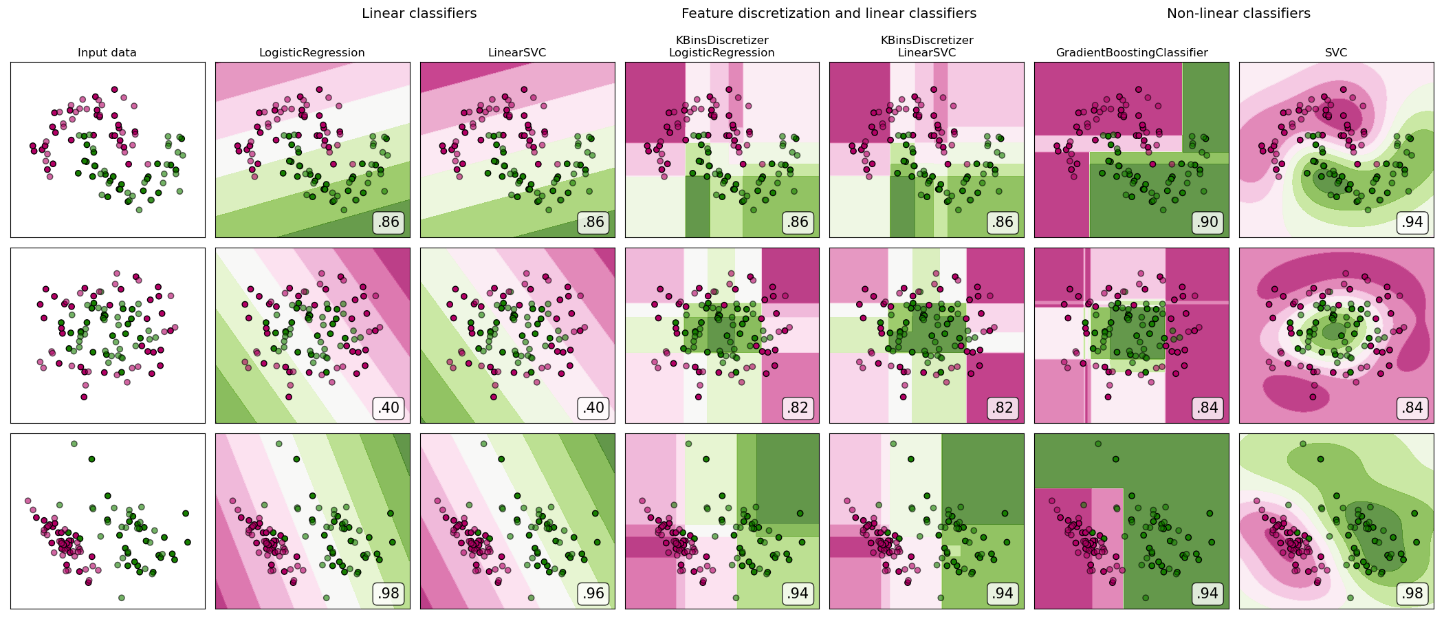
dataset 0
---------
LogisticRegression: 0.86
LinearSVC: 0.86
KBinsDiscretizer + LogisticRegression: 0.86
KBinsDiscretizer + LinearSVC: 0.86
GradientBoostingClassifier: 0.90
SVC: 0.94

dataset 1
---------
LogisticRegression: 0.40
LinearSVC: 0.40
KBinsDiscretizer + LogisticRegression: 0.82
KBinsDiscretizer + LinearSVC: 0.82
GradientBoostingClassifier: 0.84
SVC: 0.84

dataset 2
---------
LogisticRegression: 0.98
LinearSVC: 0.96
KBinsDiscretizer + LogisticRegression: 0.94
KBinsDiscretizer + LinearSVC: 0.94
GradientBoostingClassifier: 0.94
SVC: 0.98
# Authors: The scikit-learn developers
# SPDX-License-Identifier: BSD-3-Clause

import matplotlib.pyplot as plt
import numpy as np
from matplotlib.colors import ListedColormap

from sklearn.datasets import make_circles, make_classification, make_moons
from sklearn.ensemble import GradientBoostingClassifier
from sklearn.exceptions import ConvergenceWarning
from sklearn.linear_model import LogisticRegression
from sklearn.model_selection import GridSearchCV, train_test_split
from sklearn.pipeline import make_pipeline
from sklearn.preprocessing import KBinsDiscretizer, StandardScaler
from sklearn.svm import SVC, LinearSVC
from sklearn.utils._testing import ignore_warnings

h = 0.02  # step size in the mesh


def get_name(estimator):
    name = estimator.__class__.__name__
    if name == "Pipeline":
        name = [get_name(est[1]) for est in estimator.steps]
        name = " + ".join(name)
    return name


# list of (estimator, param_grid), where param_grid is used in GridSearchCV
# The parameter spaces in this example are limited to a narrow band to reduce
# its runtime. In a real use case, a broader search space for the algorithms
# should be used.
classifiers = [
    (
        make_pipeline(StandardScaler(), LogisticRegression(random_state=0)),
        {"logisticregression__C": np.logspace(-1, 1, 3)},
    ),
    (
        make_pipeline(StandardScaler(), LinearSVC(random_state=0)),
        {"linearsvc__C": np.logspace(-1, 1, 3)},
    ),
    (
        make_pipeline(
            StandardScaler(),
            KBinsDiscretizer(
                encode="onehot", quantile_method="averaged_inverted_cdf", random_state=0
            ),
            LogisticRegression(random_state=0),
        ),
        {
            "kbinsdiscretizer__n_bins": np.arange(5, 8),
            "logisticregression__C": np.logspace(-1, 1, 3),
        },
    ),
    (
        make_pipeline(
            StandardScaler(),
            KBinsDiscretizer(
                encode="onehot", quantile_method="averaged_inverted_cdf", random_state=0
            ),
            LinearSVC(random_state=0),
        ),
        {
            "kbinsdiscretizer__n_bins": np.arange(5, 8),
            "linearsvc__C": np.logspace(-1, 1, 3),
        },
    ),
    (
        make_pipeline(
            StandardScaler(), GradientBoostingClassifier(n_estimators=5, random_state=0)
        ),
        {"gradientboostingclassifier__learning_rate": np.logspace(-2, 0, 5)},
    ),
    (
        make_pipeline(StandardScaler(), SVC(random_state=0)),
        {"svc__C": np.logspace(-1, 1, 3)},
    ),
]

names = [get_name(e).replace("StandardScaler + ", "") for e, _ in classifiers]

n_samples = 100
datasets = [
    make_moons(n_samples=n_samples, noise=0.2, random_state=0),
    make_circles(n_samples=n_samples, noise=0.2, factor=0.5, random_state=1),
    make_classification(
        n_samples=n_samples,
        n_features=2,
        n_redundant=0,
        n_informative=2,
        random_state=2,
        n_clusters_per_class=1,
    ),
]

fig, axes = plt.subplots(
    nrows=len(datasets), ncols=len(classifiers) + 1, figsize=(21, 9)
)

cm_piyg = plt.cm.PiYG
cm_bright = ListedColormap(["#b30065", "#178000"])

# iterate over datasets
for ds_cnt, (X, y) in enumerate(datasets):
    print(f"\ndataset {ds_cnt}\n---------")

    # split into training and test part
    X_train, X_test, y_train, y_test = train_test_split(
        X, y, test_size=0.5, random_state=42
    )

    # create the grid for background colors
    x_min, x_max = X[:, 0].min() - 0.5, X[:, 0].max() + 0.5
    y_min, y_max = X[:, 1].min() - 0.5, X[:, 1].max() + 0.5
    xx, yy = np.meshgrid(np.arange(x_min, x_max, h), np.arange(y_min, y_max, h))

    # plot the dataset first
    ax = axes[ds_cnt, 0]
    if ds_cnt == 0:
        ax.set_title("Input data")
    # plot the training points
    ax.scatter(X_train[:, 0], X_train[:, 1], c=y_train, cmap=cm_bright, edgecolors="k")
    # and testing points
    ax.scatter(
        X_test[:, 0], X_test[:, 1], c=y_test, cmap=cm_bright, alpha=0.6, edgecolors="k"
    )
    ax.set_xlim(xx.min(), xx.max())
    ax.set_ylim(yy.min(), yy.max())
    ax.set_xticks(())
    ax.set_yticks(())

    # iterate over classifiers
    for est_idx, (name, (estimator, param_grid)) in enumerate(zip(names, classifiers)):
        ax = axes[ds_cnt, est_idx + 1]

        clf = GridSearchCV(estimator=estimator, param_grid=param_grid)
        with ignore_warnings(category=ConvergenceWarning):
            clf.fit(X_train, y_train)
        score = clf.score(X_test, y_test)
        print(f"{name}: {score:.2f}")

        # plot the decision boundary. For that, we will assign a color to each
        # point in the mesh [x_min, x_max]*[y_min, y_max].
        if hasattr(clf, "decision_function"):
            Z = clf.decision_function(np.column_stack([xx.ravel(), yy.ravel()]))
        else:
            Z = clf.predict_proba(np.column_stack([xx.ravel(), yy.ravel()]))[:, 1]

        # put the result into a color plot
        Z = Z.reshape(xx.shape)
        ax.contourf(xx, yy, Z, cmap=cm_piyg, alpha=0.8)

        # plot the training points
        ax.scatter(
            X_train[:, 0], X_train[:, 1], c=y_train, cmap=cm_bright, edgecolors="k"
        )
        # and testing points
        ax.scatter(
            X_test[:, 0],
            X_test[:, 1],
            c=y_test,
            cmap=cm_bright,
            edgecolors="k",
            alpha=0.6,
        )
        ax.set_xlim(xx.min(), xx.max())
        ax.set_ylim(yy.min(), yy.max())
        ax.set_xticks(())
        ax.set_yticks(())

        if ds_cnt == 0:
            ax.set_title(name.replace(" + ", "\n"))
        ax.text(
            0.95,
            0.06,
            (f"{score:.2f}").lstrip("0"),
            size=15,
            bbox=dict(boxstyle="round", alpha=0.8, facecolor="white"),
            transform=ax.transAxes,
            horizontalalignment="right",
        )


plt.tight_layout()

# Add suptitles above the figure
plt.subplots_adjust(top=0.90)
suptitles = [
    "Linear classifiers",
    "Feature discretization and linear classifiers",
    "Non-linear classifiers",
]
for i, suptitle in zip([1, 3, 5], suptitles):
    ax = axes[0, i]
    ax.text(
        1.05,
        1.25,
        suptitle,
        transform=ax.transAxes,
        horizontalalignment="center",
        size="x-large",
    )
plt.show()
Общее время выполнения скрипта: (0 минут 4.119 секунды)


Связанные примеры


© 2007–2026 The scikit-learn developers
Licensed under the 3-clause BSD License.
https://scikit-learn.org/1.9/auto_examples/preprocessing/plot_discretization_classification.html


